2 Karst Research Institute ZRC SAZU, Postojna, Slovenia.
Dreybrodt, W. and Gabrovsek, F. 2003. Basic processes and mechanisms governing the evolution of karst. / Speleogenesis and Evolution of Karst Aquifers 1, www.speleogenesis.net , 26 pages, re-published from: Gabrovsek, F. (Ed.), Evolution of karst: from prekarst to cessation. Postojna-Ljubljana, Zalozba ZRC, 115-154.
Abstract: Models of karstification based on the physics of fluid flow in fractures of soluble rock, and the physical chemistry of dissolution of limestone by CO2 containing water have been presented during the last two decades. This paper gives a review of the basic principles of such models, their most important results, and future perspectives.
The basic element of evolving karst systems is a single isolated fracture, where a constant hydraulic head drives calcite aggressive water from the input to the output. Non linear dissolution kinetics with order n = 4 induce a positive feedback by which dissolutional widening at the exit enhances flow rates thus increasing widening and so on until flow rates increase dramatically in a breakthrough event. After this the hydraulic head breaks down and widening of the fracture proceeds fast but even along its entire length under conditions of constant recharge. The significance of modelling such a single fracture results from the fact that an equation for the breakthrough time specifies the parameters determining the processes of early karstification. In a next step the boundary conditions for isolated fractures are varied by including different lithologies of the rock, expressed by different dissolution kinetics. This can enhance or retard karstification. Subterranean sources of CO2 can also be simulated by changing the equilibrium concentration of the solution at the point where CO2 is injected. This leads to accelerated karstification. At the confluence of solutions from two isolated tubes into a third one, mixing corrosion can release free carbon dioxide. Its effect to solutional widening in such a system of three conduits is discussed.
Although these simple models give interesting insights into karst processes more realistic models are required. Combining single fractures into two-dimensional networks models of karst in its dimensions of length and breadth under constant head conditions are presented. In first steps the Ford-Ewers' high-dip and low-dip models are simulated. Their results agree to what one expects from field observations. Including varying lithologies produces a variety of new features. Finally we show that mixing corrosion has a strong impact on cave evolution. By this effect micro climatic conditions in the catchment area of the cave exert significant influence. A common feature in the evolution of such two-dimensional models is the competition of various possible pathways to achieve breakthrough first. Varying conditions in lithologies, carbon dioxide injection or changing hydrological boundary conditions change the chances for the competing conduits.
Karst systems developing at steep cliffs in the dimensions of length and depth are characterized by unconfined aquifers with constant recharge to the water table. Modelling of such systems shows that dissolution of limestone occurs close to the water table. The widening of the fractures there causes lowering of the water table until it becomes stable when base level is reached, and a water table cave grows headwards into the aquifer. When prominent deep fractures with large aperture widths are present deep phreatic loops originate below the water table. A river or a lake on a karst plateau imposes constant head conditions at this location in addition to the constant recharge from meteoric precipitation. In this case a breakthrough cave system evolves along the water table kept stable by the constant head input. But simultaneously deep phreatic loops arise below it.
In conclusion we find that all cave theories such as those of Swinnerton (1932), Rhoades and Sinacori (1941), and the Four-state-model of Ford are reconciled. They are not contradictory but they result from the same physics and chemistry under different boundary conditions.
1. Introduction
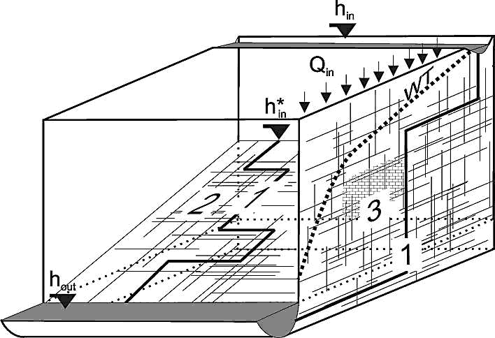
Modelling of the evolution of karst aquifers requires reduction of extremely complex systems to highly idealised simple principles. Fig.1 shows such an idealised concept of a karst system. It represents a limestone terrain with a cliff and a plateau. The limestone is dissected into blocks separated by narrow fissures and fractures. Some of those are prominent (1,2) exhibiting large aperture widths and connect water inputs at the plateau to base level at the river flowing along the foot of the cliff. They may be located along a major bedding plane parting or a master joint. Water also infiltrates from the plateau as evenly distributed seepage from meteoric precipitation and/or from a lake or stream located at the plateau. Due to such water supplies a water table is build up, where continuous dissolutional widening of fractures is activated by water containing CO2 from the atmosphere or from CO2 in the vegetated soil covering the plateau.

Fig. 1. The basic elements of a karst aquifer discussed in this work. 1: A single fracture under constant head conditions. 2: 2D fracture network under constant head conditions. 3: Vertical section of an unconfined aquifer with a constant recharge and constant head conditions applied to it. As shown, a dense network of fine fractures and a coarse network of prominent fractures are superimposed to simulate the multiple porosity character of karst aquifers. The thick dashed line WT represents the position of the water table. The hydraulic heads at the inputs and outputs are denoted as hin, h*in and hout.
Modelling the evolution of such a system in space and time needs several basic ingredients:
1. How does water flow under such conditions through the aquifer? To answer this question we must know the most simple, basic concepts of laminar and turbulent flow through single fractures or conduits.
2. Dissolutional widening depends on the dissolution rates which give the amount of limestone removed from a given area in a known time. These rates usually measured in mol cm-2s-1 can be easily converted to retreat of the wall in cm/year by a factor ![]() (Dreybrodt, 1988). They depend on many parameters. First of all on the chemical composition of the
(Dreybrodt, 1988). They depend on many parameters. First of all on the chemical composition of the ![]() solution. But also on the type of flow and on the widths of the conduits, as we will show later.
solution. But also on the type of flow and on the widths of the conduits, as we will show later.
3. Dissolutional widening changes the hydrological properties of the aquifer and alters the flow rates. Therefore flow and dissolutional widening must be coupled, to obtain the evolution in time. These basic ingredients should be combined as a first step in the most simple way by just considering one single conduit. Once the evolution of this basic element of the aquifer is known, combination of many single fractures into a complicated network becomes reasonable. Such networks are not just the sum of their ingredients. They exhibit more complex properties and these give insights into the overwhelming varieties of karst evolution.
We will lead from simple principles to more complex models, and we will try to present the most important processes active in karstification.
2. Basic Ingredients
2.1 Flow in fractures
Fig. 2 illustrates an idealised fracture with plane parallel walls separated by an aperture width ao. The width of the fracture is bo and its length is L. At the left hand side a hydraulic head h injects water into the fracture which leaves at the exit at hydraulic head zero.
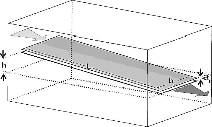
Fig. 2. Uniform fracture with aperture width a0, width b0 and length L. Calcite aggressive water is driven through it by the time-independent hydraulic head h. The goal is to calculate how do the aperture widths and flow rates evolve in time due to dissolutional widening.
For laminar flow, when each particle in the fluid follows a stable pathway, which never crosses the pathway of any other fluid particle, the flow rate Q[cm3s-1] and the hydraulic head h[cm] are related by
![]() (1)
(1)
a relation very similar to Ohm's law in electricity, which relates electric current I to voltage V by a resistance R. The resistance R for hydrodynamic flow is well known from the equation of Hagen-Poiseuille (Beek and Muttzall, 1975) and is given by
![]() (2)
(2)
![]() is the kinematic viscosity of water,
is the kinematic viscosity of water, ![]() its density, and g earth acceleration constant. M is a geometrical factor in the order of 1 and depends on the ratio a0/b0. For wide fractures a0>>bo, M=1 . For circular conduits one has a0 = b0 and M = 0.3.
its density, and g earth acceleration constant. M is a geometrical factor in the order of 1 and depends on the ratio a0/b0. For wide fractures a0>>bo, M=1 . For circular conduits one has a0 = b0 and M = 0.3.
After dissolution has changed the profile of a fracture such that the aperture width changes with distance from the entrance, R is then given by a summation over short tubes of length ![]() x, where a(x) does not change in a significant way. This can be expressed by an integral as
x, where a(x) does not change in a significant way. This can be expressed by an integral as
|
(3) |
When flow rates exceed a threshold of discharge Q flow becomes turbulent. In this case the motion of each water particle shows large fluctuations from its average flow path and also eddies will occur. As we will see later this has a significant impact on dissolution rates. The threshold when flow becomes turbulent is given by the Reynold's number ![]() , where
, where ![]() is the flow velocity in the conduit.
is the flow velocity in the conduit.
For smooth fractures and tubes flow becomes turbulent for Re > 2000. Then the relation between head and flow rate is no longer linear and the Darcy-Weissbach equation has to be applied (Dreybrodt, 1988). It reads
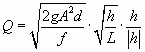 |
(4) |
where A is the cross-sectional area and d is the hydraulic diameter of the conduit. f is a friction factor given by
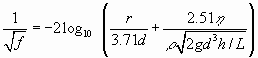 |
(5) |
r is the roughness of the wall. It is important to note that change to turbulent flow, especially in non-uniform tubes and in nets of tubes alters the distribution of heads and this puts the evolution of karst to a new stage.
2.2 Dissolution of limestone
Under conditions of karst where the pH of the solution is about 7 limestone dissolves by the reaction (Plummer et al. 1978)
|
(I) |
If no carbon dioxide is present in the solution saturation is at about 10-4 mmol/cm3. If CO2 is present the following slow reaction, enhances the solubility of calcite
|
(II) |
This process delivers a proton which removes the carbonate detached from the mineral by the reaction
|
(III) |
By this way the ion activity product ![]() is kept below the solubility constant Kc of calcite. Reactions I to III can be summarized by
is kept below the solubility constant Kc of calcite. Reactions I to III can be summarized by
|
(IV) |
Thus stoichiometrically for each CaCO3 released from the rock one molecule of CO2 is consumed by conversion to ![]() . Fig. 3 shows the equilibrium concentration of Ca++ with respect to calcite for a solution in equilibrium with a given partial pressure
. Fig. 3 shows the equilibrium concentration of Ca++ with respect to calcite for a solution in equilibrium with a given partial pressure ![]() . Under such open conditions, where each CO2 consumed is replaced by one CO2 entering from the surrounding atmosphere into the solution the equilibrium concentration is given by
. Under such open conditions, where each CO2 consumed is replaced by one CO2 entering from the surrounding atmosphere into the solution the equilibrium concentration is given by
|
(6) |
T is the temperature in °C and ![]() is in atm. This relation is valid for
is in atm. This relation is valid for ![]() atm. Mostly dissolution in early karstification proceeds under conditions closed to a surrounding atmosphere and CO2 is not replaced. In this case the CO2-concentration in the solution drops by the relation
atm. Mostly dissolution in early karstification proceeds under conditions closed to a surrounding atmosphere and CO2 is not replaced. In this case the CO2-concentration in the solution drops by the relation
|
(7) |
The straight line in Fig. 3 presents this chemical evolution towards equilibrium. Eqn. 6 is depicted by the lower curve in Fig. 3. The intersection between these two curves represents the equilibrium concentration, when the initial solution was free of Ca und in equilibrium with an initial ![]() .
.
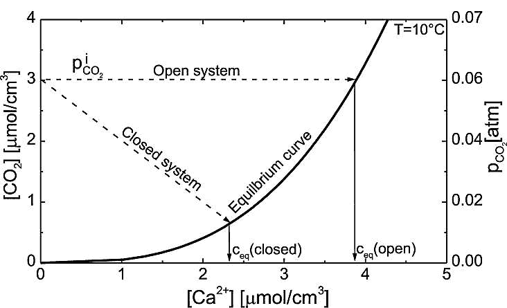
Fig. 3. Chemical pathways of solutions in the open and closed system. The thick line represents the CO2 -Ca2+ equilibrium. Dashed lines represent the pathway of solutions in the open and closed system. For each Ca2++ released one molecule of CO2 is needed. For the open system it is replaced from the CO2 – atmosphere and PCO2 stays constant. In the case of the closed system one CO2 molecule is consumed from the solution. At the intersections between the pathways and the equilibrium curve, the corresponding equilibrium concentrations can be read. The thin solid lines point to these calcium equilibrium concentration.
Dissolution of limestone in undersaturated water is controlled by three mechanisms:
1. The detachment rate at the surface of the mineral. For karst waters Plummer et al. (1978) experimentally found the following rate
![]() (8)
(8)
k3 is a constant dependent on temperature, and k4 depends also on the CO2-concentration in the solution. The first term k3 represents dissolution, the second one is the back reaction, which depends on the activities of (Ca2+)s and (![]() )s at the surface of the mineral.
)s at the surface of the mineral.
2. The ions released must be transported away from this surface into the bulk of the solution, otherwise if they would accumulate there, dissolution would stop. This transport is affected by molecular diffusion. As a consequence concentration gradients build up and the concentrations at the surface are different from those in the bulk.
3. Each ![]() detached from the mineral requires one molecule of CO2 to be reacted to
detached from the mineral requires one molecule of CO2 to be reacted to ![]() .
.
Mass conservation requires that the flux of Ca2+ from the surface must be equal to flux of Ca2+ transported into the bulk and equal to flux of CO2 towards the mineral surface. The surface dissolution rates are high, but CO2- conversion or mass transport may be rate limiting.
CO2- conversion is a slow process. For pH between 6 and 8 it takes times up to one minute until CO2 has come to equilibrium with ![]() . If water of volume V dissolves limestone from a surface area A mass conservation requires
. If water of volume V dissolves limestone from a surface area A mass conservation requires
|
(9) |
If the ratio V/A becomes small, due to the slow change of [CO2], which does not depend on V or A the rates will be limited by CO2-conversion. Note that for water flowing in a fracture with aperture width 2![]() the ratio V/A =
the ratio V/A = ![]() .
.
On the other hand if the aperture widths ![]() becomes large the diffusional resistance can also limit rates. Fig. 4 shows dissolution rates for laminar flow in an aperture under closed system conditions. The numbers on the curve give the value of
becomes large the diffusional resistance can also limit rates. Fig. 4 shows dissolution rates for laminar flow in an aperture under closed system conditions. The numbers on the curve give the value of ![]() in 10-3 cm. The rates are shown as a function of Ca, how they develop in free drift, when the solution approaches equilibrium. For small
in 10-3 cm. The rates are shown as a function of Ca, how they develop in free drift, when the solution approaches equilibrium. For small ![]() , e.g. 10-4 cm the rates are very low. This is the region where CO2 conversion is rate limiting. When
, e.g. 10-4 cm the rates are very low. This is the region where CO2 conversion is rate limiting. When ![]() increases they first increase linearly with
increases they first increase linearly with ![]() provided the Ca-concentration is kept constant. With increasing
provided the Ca-concentration is kept constant. With increasing ![]() the rates approach a limit, where they become almost independent of
the rates approach a limit, where they become almost independent of ![]() in the region of
in the region of ![]() cm to 10-1 cm. This is of high relevance since this region covers the dimension of initial fracture aperture widths in the early evolution of karst.
cm to 10-1 cm. This is of high relevance since this region covers the dimension of initial fracture aperture widths in the early evolution of karst.
All the curves in Fig.4 can be reasonably well approximated by
|
(10) |
The kinetic constant ![]() [cms-1] is in the order of 10-5 cms-1 and is listed elsewhere (see Dreybrodt 1988, Buhmann and Dreybrodt 1985). If
[cms-1] is in the order of 10-5 cms-1 and is listed elsewhere (see Dreybrodt 1988, Buhmann and Dreybrodt 1985). If ![]() >1cm mass transport becomes rate limiting and the rates are given by
>1cm mass transport becomes rate limiting and the rates are given by
 |
(11) |
where ![]() is the kinetic constant at the limit and D is the constant of diffusion for Ca2+ ( 10-5 cm2s-1). With
is the kinetic constant at the limit and D is the constant of diffusion for Ca2+ ( 10-5 cm2s-1). With ![]() cms-1 the rates are reduced by a factor of 2 for
cms-1 the rates are reduced by a factor of 2 for ![]() cm.
cm.
Fig. 4. Dissolution rates from the theoretical model for a free drift run under the conditions of a system closed to CO2. The numbers on the curves denote the values of ![]() , i.e, half the distance between the parallel calcite surfaces in 10-3 cm. For
, i.e, half the distance between the parallel calcite surfaces in 10-3 cm. For ![]() = 5*10-3 and
= 5*10-3 and![]() =1*10-1 the curves are identical. The uppermost curve gives the rates for fully turbulent motion and
=1*10-1 the curves are identical. The uppermost curve gives the rates for fully turbulent motion and ![]() =1cm. The insert in the upper right depicts the geometry of the fracture.
=1cm. The insert in the upper right depicts the geometry of the fracture.

Fig. 5. Dependence of dissolution rates on saturation ratio c/ceq.
In the early state of karstification flow is laminar, and as we will see later, after short distances of flow away from the entrance the solution comes very close to equilibrium. Close to equilibrium as has been shown experimentally (Svensson and Dreybrodt 1992, Eisenlohr et al, 1997, Dreybrodt and Eisenlohr, 2000) natural calcite carbonates exhibit inhibition of dissolution rates due to impurities in the limestone (e.g. phosphate or silicates). Then the dissolution rates drop by orders of magnitude to a non-linear rate law.
The dissolution rates for limestone are therefore given by
|
(12) |
|
|
(13) |
n varies between 3 and 6 and cs between 0.7ceq and 0.9ceq. It should be noted here that gypsum rocks follow a similar rate law (Jeschke et al, 2001) and that gypsum karst therefore can be modelled the same way as karst in limestone. In the following we use as representative numbers, ![]() , n = 4, cs = 0.9ceq, and
, n = 4, cs = 0.9ceq, and![]() for limestone. It must be stressed here that the values of
for limestone. It must be stressed here that the values of ![]() are constant only for aperture widths from about cm to 1 mm. According to Eqn.11 they drop for
are constant only for aperture widths from about cm to 1 mm. According to Eqn.11 they drop for ![]() cm, as long flow stays laminar. The rate constants kn are properties of the mineral’s surface, solely. Due to inhibition the non linear surface rates close to equilibrium are so low that they become rate limiting. Fig. 5 represents Eqns. 12 and 13. The vertical line separates the region of linear kinetics (n=1) from that of the non linear kinetics . The dotted line extends the rates of linear kinetics into the non linear region. This visualises the steep drop of inhibited non linear rates in comparison to the linear kinetics.
cm, as long flow stays laminar. The rate constants kn are properties of the mineral’s surface, solely. Due to inhibition the non linear surface rates close to equilibrium are so low that they become rate limiting. Fig. 5 represents Eqns. 12 and 13. The vertical line separates the region of linear kinetics (n=1) from that of the non linear kinetics . The dotted line extends the rates of linear kinetics into the non linear region. This visualises the steep drop of inhibited non linear rates in comparison to the linear kinetics.
When the flow becomes turbulent the bulk of the solution is mixed by the eddies, such that concentration gradients are levelled out. The completely mixed bulk is separated from the surface of the limestone by a diffusion boundary layer (DBL) of thickness ![]() . Mass transport from the mineral’s surface into the bulk and vice versa is affected by molecular diffusion through this layer. The thickness of DBL depends on the hydrodynamic conditions of flow and is given by
. Mass transport from the mineral’s surface into the bulk and vice versa is affected by molecular diffusion through this layer. The thickness of DBL depends on the hydrodynamic conditions of flow and is given by
|
(14) |
![]() is the dimensionless Sherwood number given by (Incropera and Dewitt, 1996),
is the dimensionless Sherwood number given by (Incropera and Dewitt, 1996),
|
(15) |
Re is Reynolds number, ![]() is the friction factor and
is the friction factor and ![]() is the Schmidt number
is the Schmidt number![]() . For water
. For water ![]() . The resistance to mass transport through the boundary layer is determined also by conversion of CO2. When the diffusion length of
. The resistance to mass transport through the boundary layer is determined also by conversion of CO2. When the diffusion length of ![]() -ions (i.e. the distance a
-ions (i.e. the distance a ![]() -ion travels from the mineral’s surface until it is converted to
-ion travels from the mineral’s surface until it is converted to ![]() (
(![]() )) is small compared to
)) is small compared to ![]() then diffusion is rate limiting and the effective rate constant k drops with increasing
then diffusion is rate limiting and the effective rate constant k drops with increasing ![]() . If
. If ![]() than CO2 conversion becomes rate limiting because it is affected mainly in the boundary layer. Therefore k becomes constant. Detailed numbers are given by Liu and Dreybrodt (1997).
than CO2 conversion becomes rate limiting because it is affected mainly in the boundary layer. Therefore k becomes constant. Detailed numbers are given by Liu and Dreybrodt (1997).
The thickness of the boundary layer Eqn. 14 in our calculations was in the order of several tenth of a mm. Therefore values of ![]() were used.
were used.
3. Early karstification of confined aquifers
3.1 One-dimensional conduits at constant head
As the first basic building block to understand early karst processes, we go back to Fig. 2, which represents some fractures, e.g. a bedding parting. Fig. 6 represents a part of this fracture between x and ![]() , where x is the distance from the entrance.
, where x is the distance from the entrance.
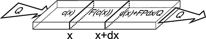
Fig. 6. Mass conservation in the part of the fracture between x and x+dx
The widening rate can be calculated by use of Eqns. 12 and 13 everywhere in the fracture if the concentration c(x) along the fracture is known. This can be found as follows. The amount of calcium dissolved from the walls per time unit must be equal to the difference of the amount of calcium entering at x to that leaving at x + dx, also related to one time unit. From this we obtain the mass balance equation
|
(16) |
where A(x) is the cross-sectional area at x, P(x) the corresponding perimeter and v the velocity. Due to the continuity of flow the constant flow rate Q through the fracture is given by ![]() .
.
Eqn.16 can be solved if one uses the dissolution rates given in Eqns.12 and 13. (Dreybrodt 1996; Dreybrodt and Gabrovsek 2000; Gabrovsek 2000). The solutions are
 |
(17) |
|
|
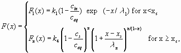
cin is the calcium concentration at the input, P is the perimeter, and xs is the position where the linear kinetics switches to the non-linear one. Fig. 7 illustrates these solutions. It shows the dissolution rates along a fracture of 1 km length for standard values given in table 1.The solid line shows the dissolution rates for linear kinetics valid up to equilibrium. Note the steep decay in dissolution rates by ten orders of magnitude in the first 5 m of the fracture. Due to such steep exponential decay the rates have dropped to ![]() after the solution has penetrated for 10m, this corresponds to dissolutional widening of 10-19 cm/year. Only surface denudation could result then.
after the solution has penetrated for 10m, this corresponds to dissolutional widening of 10-19 cm/year. Only surface denudation could result then.
The dotted lines show the dissolution rates for various n after the rate law has switched to non linearity. Here the rates drop much slower in a hyperbolic way and sufficient dissolution is still active at the exit to widen the fracture with a = 0.02cm to 0.04cm in about 100000 y, a geologically realistic time.

Fig. 7. Dissolution rates along the uniform ”standard” fracture for various orders n of the rate equation as denoted in the figure.
The evolution of the fracture widths can now be approached in the following way. In reality a funnel like profile is created because the rates at the input are higher than those at the exit. To a first approach we assume, however, that the rates at the exit are active all along the entire fracture thus maintaining a profile of parallel planes. For this we can use the analytical solutions of Eqn.16. Widening in the fracture is even and given by
![]() (18)
(18)
with
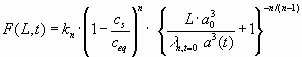 (19)
(19)
For most relevant cases, when the inflowing solution has a calcium concentration below xs the summand 1 in the bracket can be safely neglected and Eqn. 18 can be integrated after inserting Eqn. 19. The result is
|
(20) |
with
|
(21) |
Inserting the equation for F(L,0) we obtain the relation:
 |
(22) |
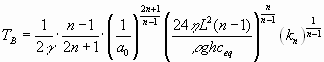
The evolution a(t) is illustrated by Fig. 8. Initially a slow increase is observed. But increasing a(t) creates increasing dissolution rates at the exit and vice versa. This positive feedback loop then finally creates the steep increase in a(t) and correspondingly in flow rate Q through the fracture.
One point is of utmost importance. The breakthrough time TB in Eqn. 22 contains the parameters which determine the time scale of early karstification. TB increases drastically with decreasing aperture width (exponent ![]() ), it increases also with L (exponent
), it increases also with L (exponent ![]() ). The dependence on head h is less drastic (exponent
). The dependence on head h is less drastic (exponent ![]() ). A most important chemical parameter is ceq. For bare karst areas, when rainwater with atmospheric
). A most important chemical parameter is ceq. For bare karst areas, when rainwater with atmospheric ![]() enters into the fractures ceq under closed condition is at about 10-4 mmol/cm3, in contrast to
enters into the fractures ceq under closed condition is at about 10-4 mmol/cm3, in contrast to ![]() mmol/cm3 in vegetated areas. This increases breakthrough times by at least one order of magnitude.
mmol/cm3 in vegetated areas. This increases breakthrough times by at least one order of magnitude.
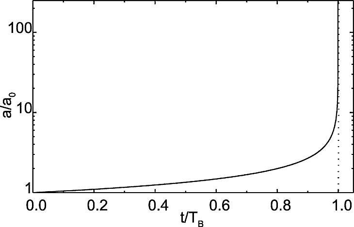
Fig. 8. Evolution of fracture aperture widths at the exit as given by Eqn.14. The dotted vertical line represents the pole of the function a(t).
The above considerations are only approximative. Numerical solutions of the equations are more exact. Fig. 9 shows the result of digital modelling of our standard case. Its parameters are listed in Table 1.
TABLE 1 Parameters used for the model of the evolution of a single fracture
| Description | Name | Unit | Initial or Standard value |
| Aperture width | a0 | cm | 0.02 |
| Fracture length | L | cm | 10 5 |
| Fracture width | b0 | cm | 100 |
| Hydraulic gradient | i | 0.05 | |
| Order of non linear kinetics | n | 4 | |
| Linear kinetics constant | k1 | ||
| Non linear kinetics constant | kn | ||
| Concentration of calcium | c | ||
| Switch concentration | cs | ||
| Equilibrium concentration | ceq | ||
| Viscosity of the solution | |||
| Density of the solution | 1 |
Fig. 9a in a logarithmic plot depicts as a function of time the flow rate through an initially plane parallel fracture with initial parameters as given in Table 1. The flow rate exhibits a slow increase that is enhanced in time until it is drastically accelerated to such an amount that they exceed the water available at the surface. At this breakthrough time TB the hydraulic head breaks down, and the initial phase of laminar flow through the fracture is terminated. Fig. 9b represents the evolution of the aperture widths along the fracture for various times depicted by points 1 to 9 in Fig. 9a. The widening rates (![]() ) are shown by Fig. 9c. In the beginning where the fracture widths at the entrance (2-4) are below 1mm the rates are given by Eqns. 12 and 13. They are maximal at c=0. Later when the entrance widens, molecular diffusion becomes rate-limiting (cf. Eqn. 11) and the rates close to the entrance drop. But they rise downstream as the aperture widths decrease. Finally when 4th order nonlinear kinetics becomes active rates are determined by Eqn.13 and they drop again. After breakthrough when flow is turbulent (dashed lines) the rates become high and even along the conduit. Details of this dynamic behaviour are given in the literature. (Dreybrodt, 1988, 1990, 1996; Dreybrodt and Gabrovsek, 2000). Fig. 9d shows the saturation ratio c/ceq along the fracture. At the beginning the ratio rises steeply until c=cs where the higher kinetics become active causing a further slow increase. With increasing flow rate the region of first order kinetics (c<cs) penetrates downstream until at breakthrough the concentration drops drastically.
) are shown by Fig. 9c. In the beginning where the fracture widths at the entrance (2-4) are below 1mm the rates are given by Eqns. 12 and 13. They are maximal at c=0. Later when the entrance widens, molecular diffusion becomes rate-limiting (cf. Eqn. 11) and the rates close to the entrance drop. But they rise downstream as the aperture widths decrease. Finally when 4th order nonlinear kinetics becomes active rates are determined by Eqn.13 and they drop again. After breakthrough when flow is turbulent (dashed lines) the rates become high and even along the conduit. Details of this dynamic behaviour are given in the literature. (Dreybrodt, 1988, 1990, 1996; Dreybrodt and Gabrovsek, 2000). Fig. 9d shows the saturation ratio c/ceq along the fracture. At the beginning the ratio rises steeply until c=cs where the higher kinetics become active causing a further slow increase. With increasing flow rate the region of first order kinetics (c<cs) penetrates downstream until at breakthrough the concentration drops drastically.
To elucidate the mechanisms of the feedback loop Fig. 9e depicts the head distribution along the fracture. In the beginning when the profile is even a(x)=a0 there is a linear decline from h to zero. The funnel shaped profile at later times distorts this decline. In the widened parts the head becomes close to the boundary value h, and at the bottleneck h declines from this value to zero at the output. Thus the hydraulic gradient increases as this bottleneck becomes shorter. Consequently flow velocity increases and dissolution rates at the exit are enhanced. After breakthrough flow becomes turbulent and the head distribution changes (dashed curves) and the decline along the fracture becomes more even. This is also important for 2 or 3-dimensional nets, because after breakthrough this new distribution of heads determines the further evolution of the aquifer.
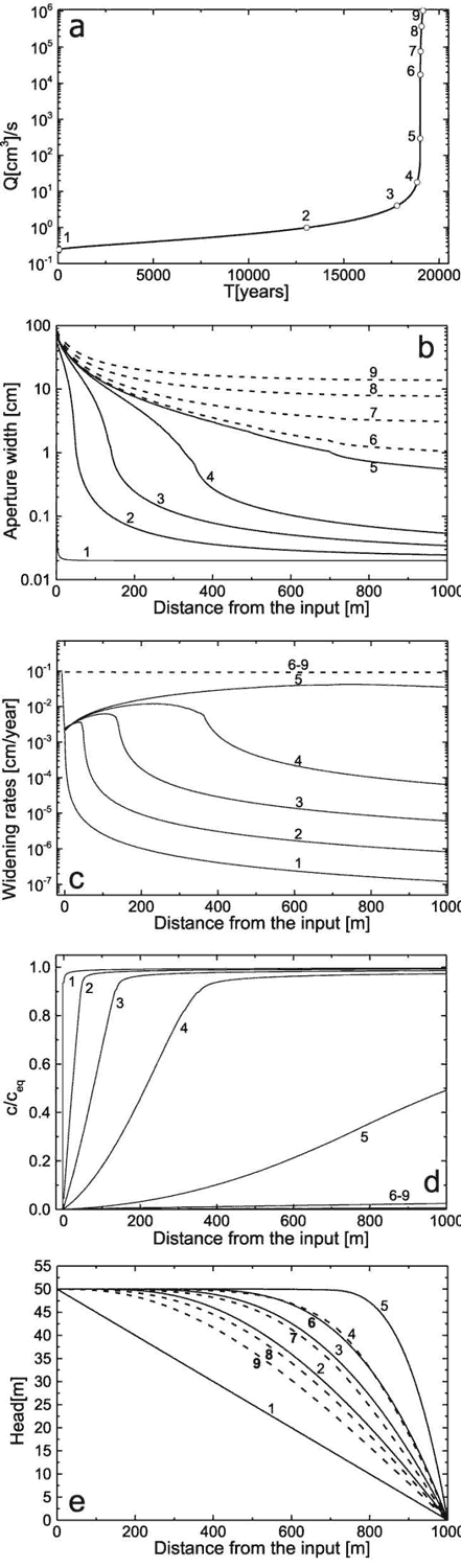
Fig. 9. Evolution of a single fracture. a) Evolution of the flow rate as a function of time. Open circles mark the points where the profiles in Figs. 9b-9e are shown. The steep increase of the flow rate marks breakthrough time. Note the logarithmic scale on Q(t). b) Profiles of the aperture widths a(x) recorded at various times: 0,13.1ky, 17.8ky, 18.85ky, 19.01ky, 19.014ky, 19.032ky, 19.082ky, 19.152ky, labeled from 1-9 respectively. Full lines indicate laminar flow and dashed lines turbulent flow. c) Dissolution rates along the fracture at times given above. d) Concentration profiles. e) Distribution of hydraulic heads along the fractures at the given times.
So far we have considered that the inflowing solution is allogenic water far away from equilibrium with respect to calcite. We now ask the question: What happens if the inflowing solution is closer to equilibrium. To answer this we consider Eqn. 17, which gives the dissolution rates along a plane parallel fracture. When cin approaches ceq, the penetration length ![]() approaches infinity and the rates become almost constant along the entire fracture, close to the maximal value at the input. Further increase in flow, will further increase the value of
approaches infinity and the rates become almost constant along the entire fracture, close to the maximal value at the input. Further increase in flow, will further increase the value of ![]() without significant influence to the rates. The reason is that the second term in the bracket of Eqn.17 becomes small with respect to the summand 1. Therefore one expects that the feedback loop gradually looses influence when cin approaches ceq.
without significant influence to the rates. The reason is that the second term in the bracket of Eqn.17 becomes small with respect to the summand 1. Therefore one expects that the feedback loop gradually looses influence when cin approaches ceq.
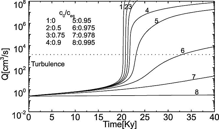
Fig. 10. The evolution of flow rate in the standard fracture for various values of c0/ceq as denoted in the figure.
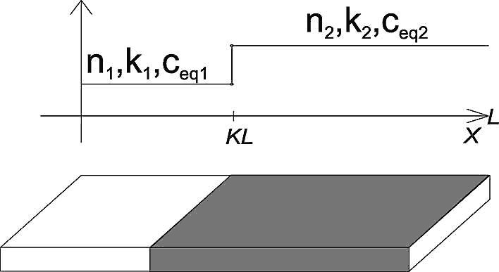
Fig. 11. Conceptual model of a heterogeneous fracture with change of kinetic properties (n,kn) or equilibrium concentration at x=KL.
This is shown by Fig. 10. It depicts the flow rates versus time for a single conduit with differing input concentrations. Curves 1 to 5, with input concentrations equal or below 0.95ceq, clearly exhibit breakthrough behaviour. When cin comes closer to ceq as in curve 6 (cin = 0.975ceq) flow rates increase steadily because dissolutional widening becomes even along the entire tube at maximal possible rate ![]() during the entire time of evolution. In that case karstification becomes very slow, but it may create horizons of increased permeability, which later, when geological conditions change may be utilised for conduit growth. Such horizons have been suggested by Lowe and Gunn (1997).
during the entire time of evolution. In that case karstification becomes very slow, but it may create horizons of increased permeability, which later, when geological conditions change may be utilised for conduit growth. Such horizons have been suggested by Lowe and Gunn (1997).
3.2 The heterogeneous fracture
In the examples discussed up to now all chemical parameters ceq , kn , n and k1 were assumed as constant along the entire fracture length. This is highly idealistic. In nature karst conduits may have sections of varying lithology and therefore with varying values of n and kn. Subterranean sources of CO2 could enter into fractures and increase the solubility of limestone reflected by an increase of ceq. In this section we will shortly discuss the influence of such new conditions on breakthrough time (Gabrovsek et al., 2000, Gabrovsek, 2000).
Fig. 11 depicts the heterogeneous standard fracture, which exhibits different properties, such as different dissolution kinetics or differing ceq, in its entrance part for ![]() and the exit region for
and the exit region for ![]() .
.
First we assume differing dissolution kinetics with ![]() and
and ![]() in the first half of the fracture (K = 0.5) and
in the first half of the fracture (K = 0.5) and ![]() and
and ![]() in the remaining part.
in the remaining part.
Fig. 12 shows the numerical results for the standard fracture with ![]() and
and ![]() (a,b,c) and for the reverse case, when
(a,b,c) and for the reverse case, when ![]() and
and ![]() (d,e,f). Both fractures show breakthrough behaviour, but at quite different time scales.
(d,e,f). Both fractures show breakthrough behaviour, but at quite different time scales.
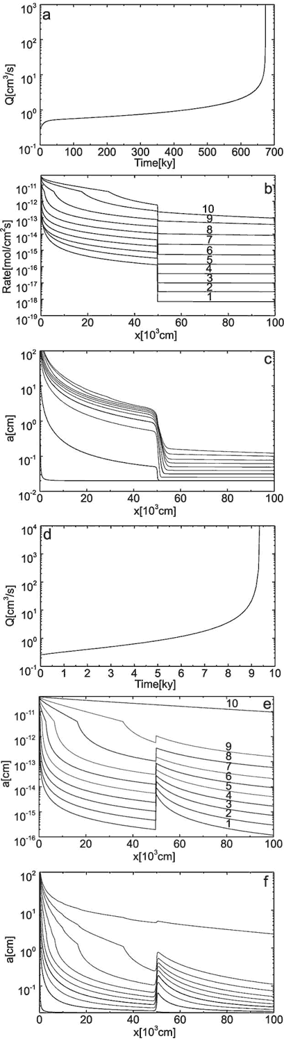
Fig. 12. a) Evolution of flow rates in time for the standard fracture with n1 = 4, n2 = 6 and K = 0.5 (b,c) Profiles of dissolution rates and aperture widths for n1 = 4, n2 = 6 and K = 0.5 plotted at 0.1, 45.8, 452.1, 599.4, 649.1, 665.5, 670.9,672.5, 673 and 673.1ky marked from 1-10 respectively. d) Evolution of flow rate in time for the standard fracture with n1 = 6, n2 = 4 and K = 0.5. e,f) Profiles of dissolution rates and aperture widths for n1 = 6, n2 = 4 and K = 0.5 at 0.1, 3.3, 5.8, 7.3, 8.2, 8.7,9, 9.2, 9.3 and 9.4 ky marked from 1-10 respectively.
For n1 < n2 the dissolution rates drop drastically when the solution encounters the border of changing lithology. Since the solution is close to saturation the dissolution rates, shown by Fig. 12b, remain constant from then on. After the time of 45ky the first half of the fracture has opened up to such an extent that the hydraulic head remains close to the input head and the head loss from h to base level zero is along the second half. With increasing widths of this half flow rates increase such that the concentration at the boundary becomes sufficiently high to switch on the feed back loop causing breakthrough. Breakthrough time is greatly influenced by the low dissolution rates at the exit of the fracture and is substantially longer than in the homogeneous standard fracture (cf. Fig. 9).
For ![]() and
and ![]() (Fig. 12 d-f) the dissolution rates are boosted up when the solution meets the border. Due to the significantly lower dissolution rates in the entrance half the concentrations remain sufficiently high such that breakthrough is dominated by the kinetics with
(Fig. 12 d-f) the dissolution rates are boosted up when the solution meets the border. Due to the significantly lower dissolution rates in the entrance half the concentrations remain sufficiently high such that breakthrough is dominated by the kinetics with ![]() in the exit part. Compared to the first case the initial rates at the exit are higher by two orders of magnitude. Therefore breakthrough time is only 10ky, even less than that of the standard fracture. These examples show that differing lithologies have a strong impact on karstification and cannot be neglected. More details on this issue are reported by Gabrovsek (2000), and by Dreybrodt and Siemers (2000).
in the exit part. Compared to the first case the initial rates at the exit are higher by two orders of magnitude. Therefore breakthrough time is only 10ky, even less than that of the standard fracture. These examples show that differing lithologies have a strong impact on karstification and cannot be neglected. More details on this issue are reported by Gabrovsek (2000), and by Dreybrodt and Siemers (2000).
We now turn to the case where ceq changes step like by injection of subterranean carbon dioxide. Fig. 13 shows the numerical results of the dissolution rates along the standard fracture for two cases. a) K = 0.25 and b) K = 0.75. At these positions ![]() mol/cm3 increases by
mol/cm3 increases by ![]() mol cm-3. With an increase of
mol cm-3. With an increase of ![]() the rates are enhanced, where CO2 is injected into the fracture and consequently dissolutional widening becomes faster there. The fracture profiles are depicted by Fig. 14 for both cases. Fig. 15 illustrates the breakthrough behaviour for the cases K=1 (standard fracture), K = 0.25 (Fig. 14a), K = 0.75 (Fig. 14b), and K = 0.9. In all cases of CO2 - injection breakthrough times are reduced. Further details are published by Gabrovsek et al. (2000). It should be noted here that also injection of solutions with different chemical composition can increase ceq e.g. mixing corrosion, and reduce breakthrough times.
the rates are enhanced, where CO2 is injected into the fracture and consequently dissolutional widening becomes faster there. The fracture profiles are depicted by Fig. 14 for both cases. Fig. 15 illustrates the breakthrough behaviour for the cases K=1 (standard fracture), K = 0.25 (Fig. 14a), K = 0.75 (Fig. 14b), and K = 0.9. In all cases of CO2 - injection breakthrough times are reduced. Further details are published by Gabrovsek et al. (2000). It should be noted here that also injection of solutions with different chemical composition can increase ceq e.g. mixing corrosion, and reduce breakthrough times.
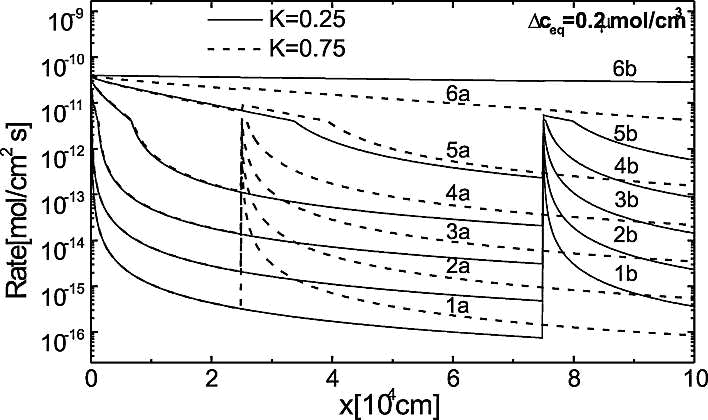
Fig. 13. Dissolution rates for the point CO2 input at K=0.25 (dashed lines) recorded at 0.1, 6.5, 9.4, 10.13, 10.35, 10.39 ky (labeled from 1a to 6a respectively) and the for the input at K=0.75 (full lines) recorded at 0.1, 6.93, 10.19, 11.07, 11.27, 11.31 ky (labeled from 1b to 6b respectively).
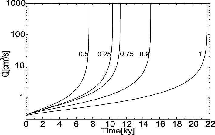
Fig. 15. Breakthrough times for the standard fracture with CO2-input at to x=KL for various values of K.
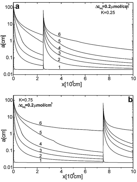
Fig. 14. a) Profiles of aperture widths for the input of CO2 at K=0.25, recorded at the times given in Fig. 13, labeled from 1-6. b) Profiles of aperture widths for the input of CO2 at K=0.75, recorded at the times given in Fig. 13, labeled from 1-6.
3.3 Evolution of caves in 2-dimensional nets of fractures
To approach further to reality we consider a confined aquifer consisting of a limestone bed dipping downward, which is dissected by narrow initial fractures. This is shown schematically by the model domain in Fig. 16. The bed dips from left to right. The left hand side has input points, where the head and the chemical composition of the inflowing water can be defined individually for each input point. The left hand side is at base level, i.e. h=0. The aperture width of each fracture can be assigned individually. By this way it is possible to model the statistical properties of fracture widths. In the following we use a log-normal distribution of fracture widths with average and . It is also possible to use bi-modal distributions to simulate a coarse net of wide fractures embedded into a dense net (continuum) of narrow fractures to account for the double-porosity properties of karst aquifers (Sauter, 1992).
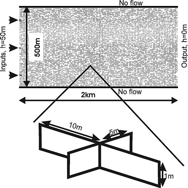
Fig. 16. Modelling domain of its 2-dimensional fracture network. The length of the domain is 2km, the width 500m. Fracture spacing is 10m x 5m. Each fracture has uniform initial aperture width, which is determined by a log-normal distribution over the entire set of fractures. There are three inputs on the left side of the domain at h=50 m and a series of outputs on the right hand side at h=0.
To model the evolution of conduits in such nets one has to calculate the distribution of hydraulic heads at all the nodes in the net and from these the flow rate through each fracture. Furthermore one must know the chemical composition of the solution at each node to couple the flow to the chemical dissolution model in each single fracture. Technical details of this procedure are described by Siemers and Dreybrodt (1998) and by Gabrovsek (2000). The parameters of the model domain are ![]() cm,
cm, ![]() cm, h = 50 m, the length L of the domain is 2km and its width 500 m. The upper and the lower boundaries are impermeable.We first apply our modelling efforts to the high-dip model of Ford and Ewers (see Ford and Williams, 1989). Fig. 17 shows the evolution with 3 inputs with equal chemical composition and equal heads.
cm, h = 50 m, the length L of the domain is 2km and its width 500 m. The upper and the lower boundaries are impermeable.We first apply our modelling efforts to the high-dip model of Ford and Ewers (see Ford and Williams, 1989). Fig. 17 shows the evolution with 3 inputs with equal chemical composition and equal heads.
Fig. 17a depicts the situation after 8000 years. Several conduits have grown downstream. At approx. 17590 (Fig. 17b) years the upper has reached base level and breakthrough occurs. Therefore the constant head boundary condition at this input is replaced by a constant flow rate at that input. Thus the hydraulic head in this conduit drops to values close to base level, as can be seen from the pressure isolines in the figures. This directs flow from the conduits which have not reached base level towards the master conduit. Therefore they integrate into a common system. When such a conduit reaches the leading one breakthrough occurs (Fig. 17c and d) and again the constant head condition at the input is changed to constant flow. The distribution of flow rates within the network is illustrated by Fig. 19.
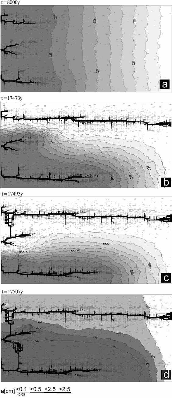
Fig. 17. Distribution of aperture widths and hydraulic head isolines at various times for the domain presented in Fig.16. Hydraulic head at the left hand side is set to 50m and 0 at the right-hand side. Water at all inputs is in equilibrium with pCO2=0.05atm. All fractures smaller than 0.05 cm have been omitted. The bar code indicates the numerical values.
The rates are depicted in units of Qmax which is the maximal flow rate through a fracture which occurs in the net. Note that Qmax increases in time. As one visualises from Fig. 19a flow is widely distributed over the net initially. As the conduits grow down head the flow is radiating into the net from their tips. After breakthrough flow is concentrated in the mayor conduits (Figs. 19b-d). The evolution of the flow rates through the aquifer is depicted by Fig. 18 (curve1), which also shows the subsequent break through events. This scenario shows a competition between the growing conduits. Prior to breakthrough each of these propagates down head. The breakthrough time for such single 1-dimensional channels is therefore similar as in Eqn. 22, where a0 has to be replaced by the average initial aperture width along the conduit and L must be replaced by its total length. Since these values, due to the statistical distribution of fracture widths are different for each of the evolving conduits the one with shortest breakthrough time wins the race. Siemers and Dreybrodt (1998) have shown by a sensitivity analysis to the various parameters that Eqn.22 is applicable for the breakthrough time in two-dimensional nets under constant head conditions. It should be noted here, that the breakthrough time for a defined conduit, where length and average a0 are exactly known, can be significantly shorter, than that of an isolated one-dimensional conduit. The reason for this is that a conduit embedded into a net of fractures looses fluid into the net (see Fig. 19a,b). Therefore under constant head conditions more aggressive solution enters into this fracture and enhances dissolutional widening (Romanov et al. 2002a).
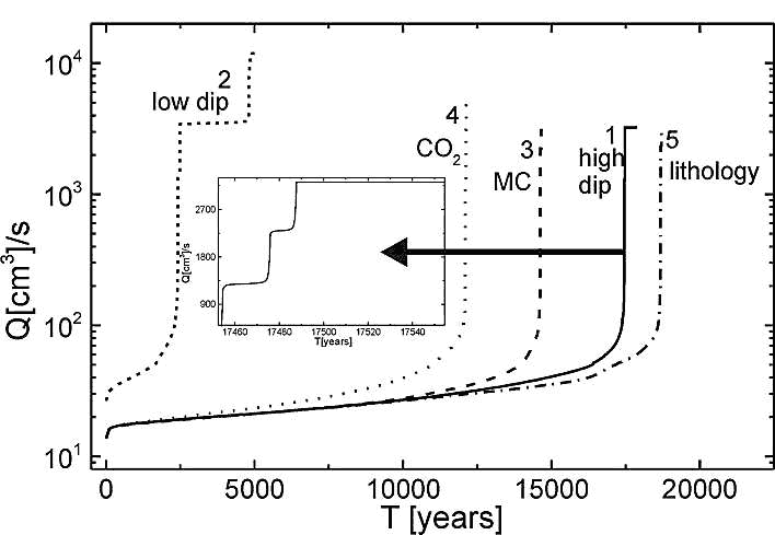
Fig. 18. Evolution of total flow through the network in time for all 2-dimensional cases. Insert shows the sequential breakthroughs in the high-dip model (Figs. 17 and 19).
As a next example we discuss the low-dip-model by Ewers and Ford. In this case two additional inputs are placed in the central section of the aquifer, both with equal heads and equal chemical composition of the solutions as those at the left hand side of the domain. This is illustrated by Fig. 20. After 2000 years (a) channels from these inputs have propagated downstream. No conduits can grow from the inputs at the left hand boundary, because these have only negligible head difference to the central region. After 2470 years (b) the conduits exhibit a breakthrough and integrate together similar as in the high dip case. This changes the hydraulic head distribution and conduits from the inputs at the left hand side grow towards these channels. Each row of inputs behaves similar as the high-dip model, and an integration of their conduit systems grows upwards (Figs. 20 c,d).

Fig. 19. Flow pattern in the network at the same times as in Fig. 17. Line’s thickneses in the bar code represent the values of Q/Qmax, where Qmax is the flow rate through the fracture with highest flow.
At each breakthrough event the constant head condition at the corresponding input is replaced by constant flow. This causes changes in the distribution of hydraulic heads, which direct growing channels towards conduits of constant flow rate, or in other words head zero. The evolution of flow rates is depicted by Fig. 18, curve 2.
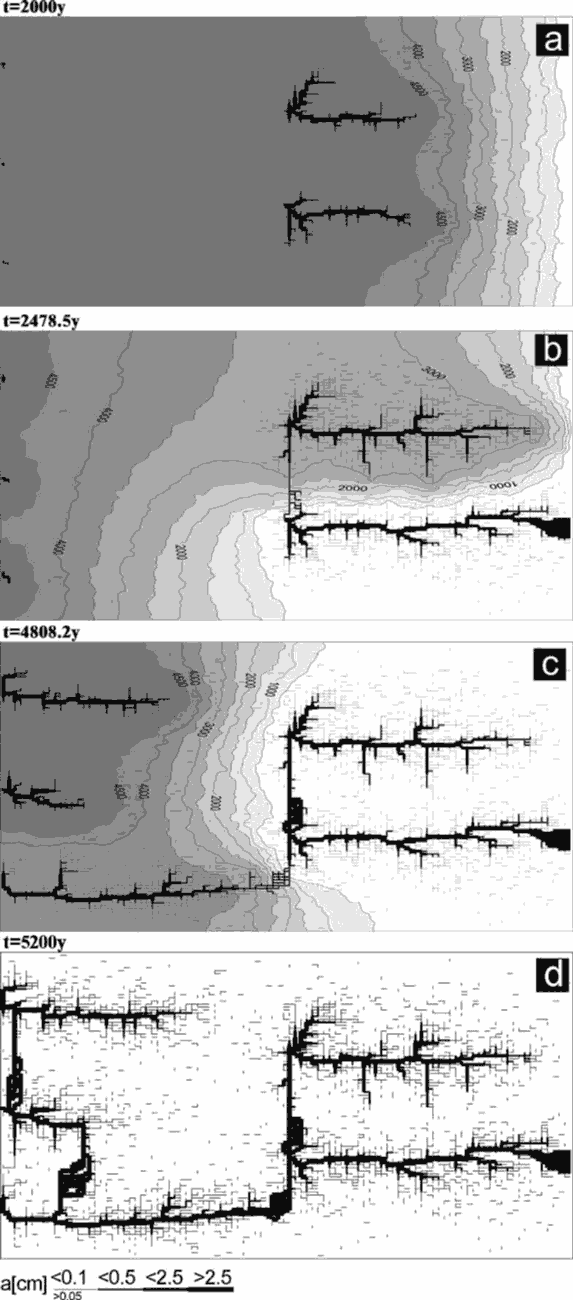
Fig. 20. Aperture widths and hydraulic heads at various time for the low-dip model. Same settings as in Fig.17, but two inputs at h=50m are added to the middle of the domain.
During the early evolution of a karst aquifer prior to breakthrough the concentrations of the solutions within the karst aquifer are very close to saturation (cf. Fig 9c, single fracture). If the chemical composition of the waters at the inputs are different with respect to initial ![]() and these waters mix somewhere within the aquifer mixing corrosion will boost up dissolution rates. To show the impact of mixing corrosion to the evolution of karst we have changed the chemical composition at the central input in the high-dip model shown by Fig. 17 and have left everything else unchanged. Fig. 21 shows the result.
and these waters mix somewhere within the aquifer mixing corrosion will boost up dissolution rates. To show the impact of mixing corrosion to the evolution of karst we have changed the chemical composition at the central input in the high-dip model shown by Fig. 17 and have left everything else unchanged. Fig. 21 shows the result.
In contrast to the evolution with equal input chemistry in Fig.17, where the outer conduits grow simultaneously, now the middle conduit has advanced significantly. The outer conduits have stopped growth at 12000y. The reason for this is that during the early phase of evolution water from the two outer inputs injected into system of narrow fractures mixes with water from the central input. Therefore dissolutional widening by mixing corrosion increases the average fracture widths to such an extent that the central conduits gain sufficient advantage to reach base level first. After breakthrough growth of the outer channels is directed towards the central one. The evolution of flow rates is shown in Fig. 18, curve 3.
This example shows that changes in the chemical parameters are of utmost importance. Changes in vegetation can alter the chemical composition of the input waters and can divert the evolving cave patterns to a high extent. By this way climate can effect cave evolution. Details on the effect of mixing corrosion are reported by Gabrovsek and Dreybrodt (2000) and Romanov et al. (2002b).
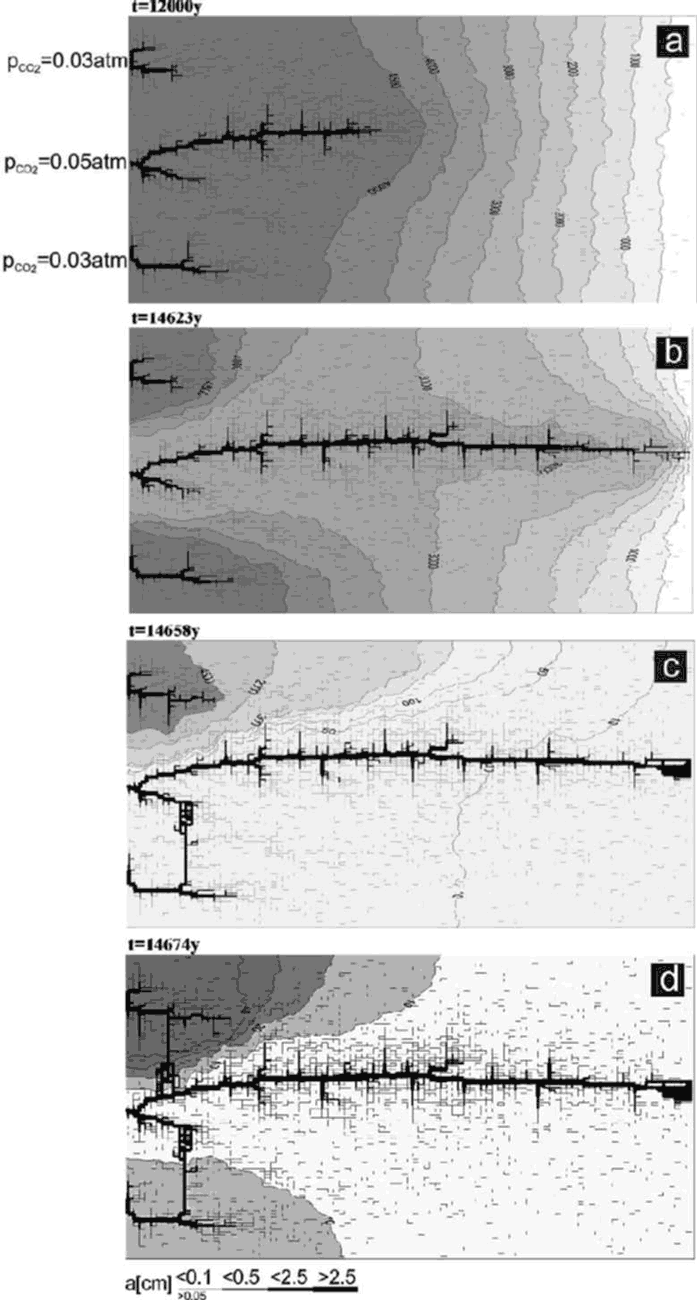
Fig. 21. Aperture widths and hydraulic heads at different times for the case with mixing corrosion. Same settings as in Fig. 17, but water at upper and lower inputs has reduced content of CO2 (pCO2=0.03)
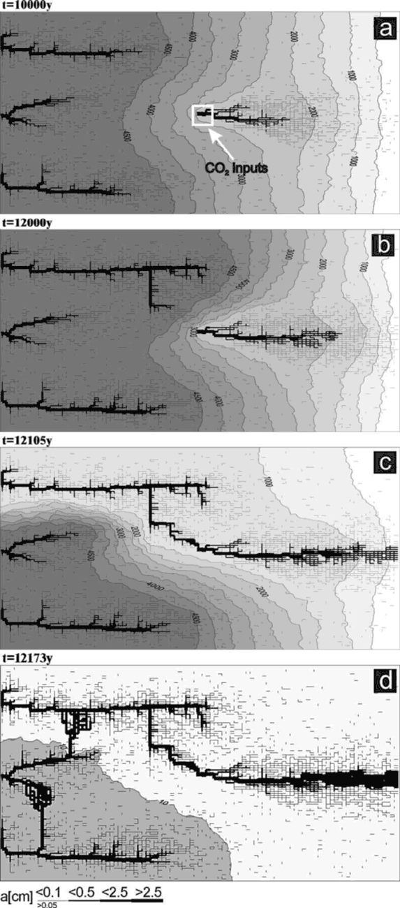
Fig. 22. High-dip model (Fig. 17) with a CO2 input. pCO2 in the region marked in Fig. 22a is set to 0.05atm.

Fig. 23. High-dip (Fig. 17) model with changing lithology. As marked in Fig. 23a, the kinetic order changes within the network from 4 to 6 and back to 4.
When subterranean sources of CO2 either by volcanic origin or by microbial activity are present in the aquifer dissolutional widening is enhanced in the regions neighbouring such inputs. Therefore these regions favour the evolution of conduits growing to their direction. Fig. 22 shows such an example. Here a point source of CO2, which raises ceq by ten percent is located in the middle of aquifer. From this input points due to the enhanced dissolution rate a channel grows down head, which is joined by the upper conduit.
Comparison of the evolution compared to that in Fig. 17 shows the strong influence of subterranean CO2 sources. This is also reflected by the evolution of the flow rates shown in Fig.18, curve 4. Further details have been published by Gabrovsek and Dreybrodt (2000).
Varying lithology can change the parameters of the dissolution kinetics (Eisenlohr et al. 1999). Fig. 23 shows the evolution of the aquifer, when its middle part is composed of limestone with ![]() whereas the outer parts remain unchanged with n=4. Due to the altered kinetics dissolutions rates in the middle part drop, when they are encountered by the solution and channels grow only in the input part with n=4. When such a channel has reached the border between the two lithologies channels grow down head until a first reaches base level and breakthrough occurs. The flow rates for this case are shown by Fig.18, curve 5.
whereas the outer parts remain unchanged with n=4. Due to the altered kinetics dissolutions rates in the middle part drop, when they are encountered by the solution and channels grow only in the input part with n=4. When such a channel has reached the border between the two lithologies channels grow down head until a first reaches base level and breakthrough occurs. The flow rates for this case are shown by Fig.18, curve 5.
4. Modelling unconfined aquifers in the dimension of length and depth
So far we have discussed confined aquifers subjected to constant head conditions. By use of this modelling concept the evolution of caves in the dimension of length and breadth can be studied. Now we project one dimension to depth to investigate cave evolution in length and depth. In this projection of reality new boundary conditions must be envisaged.
The aquifer need no longer be confined and a water table may be present. Furthermore input conditions of constant recharge must also be considered. In the following we will present the conceptual frame for such models.
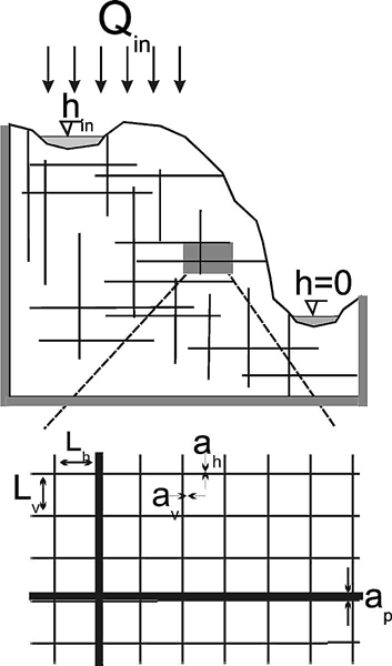
Fig. 24. Schematic representation of a cross-section through the limestone plateau. At the top a combination of constant recharge and constant head conditions can be applied. Thick grey lines show impermeable boundaries. The lower picture is an enlargement showing the parameters of the fracture systems.
Fig. 24 shows a vertical section of a limestone plateau down cut by a valley on its right-hand side. The massif is dissected by fractures of various initial aperture widths. Prominent fractures are shown in the massif. The enlargement shows a net of fine fractures that are evenly distributed throughout the aquifer. Fig. 25 shows a simplified version of the cross-section representing the modelling domain discussed in this chapter. The model plateau is rather small, 200m long and 30m high. The hydraulic conductivity represented by the rectangular net of fine fractures with aperture widths![]() is about 10-7cm/s. Prominent fractures with aperture widths in the order of few tenth of a millimetre can be incorporated into the system of narrow fractures. A recharge of 450mm/year is evenly distributed at the surface of the plateau and ”offered” to the aquifer. The left-hand side, the base and the lower right-hand side are assumed impermeable. This is marked by thick solid lines in Fig.25. The hydraulic head hout at base level is set to zero. The cliff on the right represents a seepage zone where the water leaks from the aquifer. Constant head conditions can be applied additionally on the top, e.g. an allogenic river flows over the massif. Table 2 presents the parameters used in the model and their typical values.
is about 10-7cm/s. Prominent fractures with aperture widths in the order of few tenth of a millimetre can be incorporated into the system of narrow fractures. A recharge of 450mm/year is evenly distributed at the surface of the plateau and ”offered” to the aquifer. The left-hand side, the base and the lower right-hand side are assumed impermeable. This is marked by thick solid lines in Fig.25. The hydraulic head hout at base level is set to zero. The cliff on the right represents a seepage zone where the water leaks from the aquifer. Constant head conditions can be applied additionally on the top, e.g. an allogenic river flows over the massif. Table 2 presents the parameters used in the model and their typical values.
TABLE 2: Parameters of unconfined model
| Description | Name | Unit | Standard or Initial value |
| Aperture width | a0 | cm | 0.006 |
| Aperture width of prominent fractures | ap | cm | 0.02 |
| Length of vertical and horizontal fractures | Lv, Lh | cm | 50, 200 |
| Hydraulic conductivity | K | ms-1 | 10-7 |
| Annual recharge | Q | mm/year | 450 |
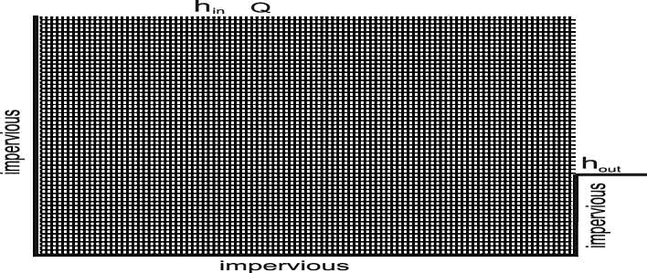
Fig. 25. The model domain with its boundary conditions.
Our model implies an unconfined aquifer, i.e. an aquifer with a water table (WT) which divides a saturated phreatic and an unsaturated vadose zone (see Fig. 1). Recharge is infiltrating through the surface and the vadose zone down to the phreatic zone at the WT. The position of the WT depends on recharge.
To obtain the flow through the fractures, the position of the WT must be known, since it defines the boundary conditions for flow and separates the saturated zone from the unsaturated one.
The position of the WT and the height of the seepage face is calculated by the following procedure:
- An initial guess for the WT is assumed, f.i. the surface of the plateau.
- A recharge defined by precipitation is equally distributed to the points of the assumed WT.
- The heads of all the net-points below and at the assumed WT are calculated with the boundary conditions defined by the assumed WT and seepage face, i.e. h=z.
- The heads of the points on the WT are checked for the boundary condition. Their head must be, within a given error, equal to their elevation. If this condition is valid for the point, the WT is kept there, otherwise the WT is either shifted to the point above, if h > z or to the point below if h < z . Thus a new approximation for the WT is obtained.
- Procedure 1-3 is iterated until all the points on the assumed WT fulfil the condition h = z.
Once the WT and the seepage zone are obtained, the flow through the fractures in the phreatic zone is calculated and the transport-dissolution model is applied. This is done in the same way as described for confined networks.
Chemical parameters used are those given in Table 1. During percolation through the vadose zone, the solution already attains some saturation state. This is taken into account by taking c0 between cs and 0.97ceq, so that the initial concentration rises linearly with the depth of the water table. The choice of the parameter c0 is rather arbitrary. It influences the evolution of an aquifer, but does not change the results conceptually. A broad sensitivity analysis has not yet been done. Details are given in Gabrovsek and Dreybrodt (2001) and in Gabrovsek (2000).
4.1 The evolution of fine fracture systems. No prominent fractures:
Constant recharge
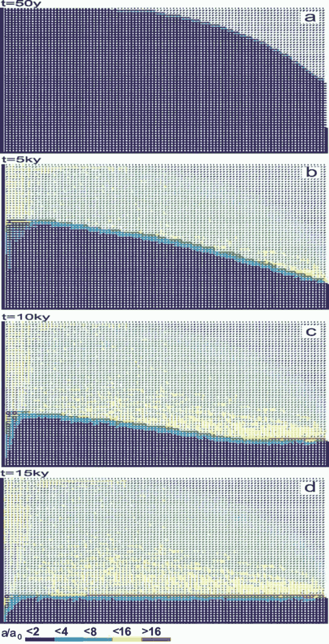
Fig.26. Evolution of an aquifer with evenly spaced fine fractures and constant recharge. Distribution of fracture widths after 50y (a), 5ky (b), 10ky (c) and 15ky (d). The colours represent the widths of the fractures in units a(t)/a0, where a0 is the initial width of vertical fractures. Fractures designated by full squares represent the phreatic zone, those by open angles the vadose zone. By this way the water table is clearly presented.
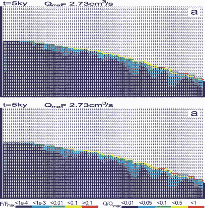
Fig. 27. a) Flow rates in units of Q/Qmax at 5ky. The fracture with the highest flow rate has a ratio of Q/Qmax equal to 1. Most of the flow is concentrated to the permeable fringe at the top of the phreatic zone. Confer to Fig.26. b) Dissolution rates in units F/Fmax where Fmax = corresponding to bedrock retreat of few . The maximal dissolution rates are active close to the water table and drop rapidly with depth.
The aquifer consists of system of narrow fractures. No prominent fractures are present in the modelling domain. We assume a constant recharge of 450mm/year evenly distributed to the surface of the plateau. Fig.26a shows the situation at the onset of karstification. The phreatic zone is indicated by fat fracture lines, and the vadose zone by thin interrupted ones. In this way the position of the WT is clearly presented. The colours show the fracture aperture widths increasing from dark blue to red as denoted in the figure. a0 is the initial width of the vertical fractures. Fig.26b shows the situation after 5ky. The WT has dropped due to the increasing fracture widths in the aquifer. After 10ky the WT reaches the lowest output fractures. This is presented in Fig.26c. By continuous dissolution along the base level a conduit develops and grows headwards (Fig.26d) until it reaches the left boundary after 20ky. Inspection of the colours in Fig.26d reveals that the hydraulic conductivity increases by about 2 orders of magnitude, leaving a highly permeable vadose zone as is observed in nature. Dissolutional widening is most active close to the water table at all times, since the solution quickly approaches equilibrium when penetrating into the net. Therefore close to the WT a narrow region of higher permeability is established which attracts flow. In Fig.26a a small light blue fringe indicates this zone.
Later the fringe becomes wider and is composed of fractures with apertures up to 16a0. With increasing time the water table drops, leaving behind the vadose region of increased conductivity. The phreatic zone below still has low hydraulic conductivity. In such an aquifer most of the flow is directed along the water table.
After 15ky the conduit at the WT has reached an average width of 1cm. The fracture widths in the vadose zone above are between 0.01-0.1cm, with the wide fractures close to the final WT.
Fig.27a shows the flow rates through the fractures at 5 ky and clearly illustrates (green, yellow, red fractures) that the flow is restricted close to the water table. Dissolution rates shown in Fig.27b also exhibit a maximum close to the water table and drop significantly below. As the water table drops dissolution becomes active in the lower parts of the aquifer. Once the water table has reached a stationary position dissolution stays active close to it and large conduits can grow. This corresponds to the ideal water table cave in the model of Swinnerton (1932) and Rhoades and Sinacori (1941) which requires high and even fissuring of the rock.
Combined conditions: constant recharge and constant head
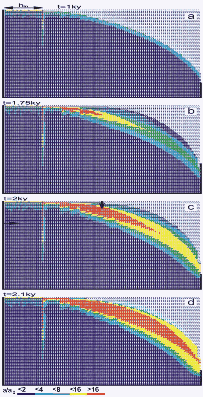
Fig. 28. Evolution of a fine fracture system with combined constant recharge and constant head conditions at the top. The constant head region is marked in figure a. The WT is fixed due to the constant head. Dissolution is mainly active in the fringe close to the water table. The arrows on figure c denote the position of the profiles presented in figure 30.
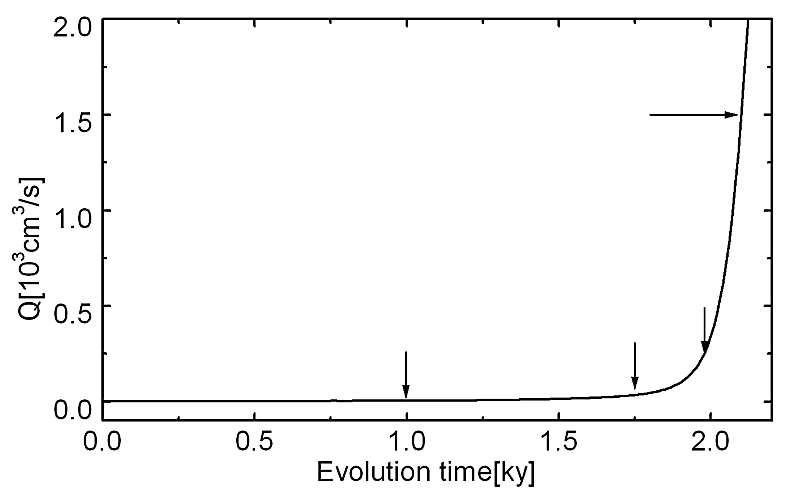
Fig. 29. Evolution of flow rate through the network in Fig.28. Arrows indicate times when aperture distributions in Fig.28 are presented.
Often constant head boundary conditions and those of constant recharge exist simultaneously. This for example is the case when allogenic rivers are present. Fig.28 shows such a case where a constant head equal to the elevation at the upper left boundary is imposed (see Fig. 28a). Other parameters are equal to those in Fig.26. Constant recharge is offered to the aquifer everywhere else. Fig.28a shows the water table and the distribution of the fracture aperture widths 1ky after the initial state. In the region of constant recharge the water table drops towards the seepage face, whereas in the condition of constant head it coincides with the surface at the platform. Dissolution occurs only in a small banded region close to the WT as illustrated by Figs.28a, b, c. In the constant head region, the water table cannot drop below the surface, therefore the head difference along the WT increases. A permeable fringe along the WT offers an effective pathway draining the water from the constant head region to the output. The feedback mechanism along this pathway leads to the breakthrough at 2.1ky. A wide zone of high conductivity has been created which carries flow from the constant head area.
Fig.29 shows the total discharge as a function of time. The arrows indicate the flow rates at the time steps from Fig.28. This resembles a typical breakthrough behaviour such as observed for one-dimensional conduits or for nets under constant head conditions. To obtain some information on the widths of the fractures Fig. 30 depicts the aperture width profiles along a vertical and horizontal cross-section as indicated by the arrows in Fig. 28c.
4.2 Aquifers with a net of prominent fractures
To create a more realistic karst aquifer we now superimpose a net of prominent fractures to the system of fine fractures. The following procedure is used:
• Divide the net of fine fractures into a coarse net of 5 by 5 dense fractures
• With a random procedure assign to each fracture of this coarse net the aperture width ap, of a prominent fracture. If the random number chosen for each fracture is smaller than p, the fracture has an aperture width ap, else its aperture is that of the fine net fractures.
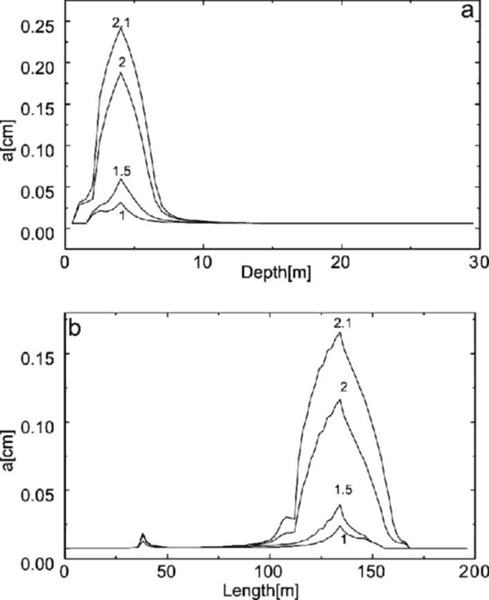
Fig. 30. Distribution of the fracture widths for a horizontal and vertical cross-section of the aquifer as indicted by arrows in Fig. 28c. The numbers on the curves indicate the time of the aquifer evolution in ky. a) Widths of the vertical fractures in the vertical cross-section for various times indicated in ky. The region of maximal widths corresponds to the red area in Fig.28. b) Widths of the horizontal fractures in the horizontal cross-section for various times. The small peak at about 30m corresponds to the vertical channel, which develops at the border between constant head and constant recharge regions. Note that the increase of aperture widths accelerates in time.
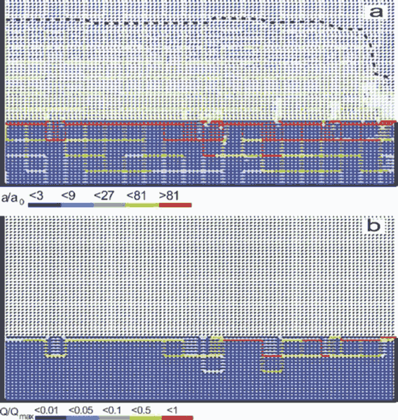
Fig. 31. Aquifer with a percolating net of prominent fractures (ap = 0.04cm). Annual precipitation is 700 mm/year. a) Distribution of fracture widths after 30ky. Conduits grow along the base level and along the phreatic loops. Note the change in the colour code with respect to other figures. The widths designated by red are above 0.5cm. The dashed line depicts the initial WT. b) Distribution of flow rates at 30ky.
This initial scenario is similar to the approach of a double continuum model of Clemens et al. (1996, 1997, 1999) but it avoids calibration parameters, which are difficult to specify. It is also close to the approach of Kaufmann and Braun (1999, 2000) whomodel the initial aquifer by a superposition of a prominent fracture net within a rock matrix with homogeneous initial conductivity. The most important difference in our approach is that dissolutional widening is regarded in both parts of the aquifer, whereas Clemens et al. and also Kaufmann and Braun disregard dissolution in the dense fractures or in the matrix respectively.
Boundary conditions of constant recharge
As pointed out dissolution in our model is active in the prominent fractures as well as in the continuum of narrow fractures. The question arises, where does permeability arise in the competition of gaining flow from the surface.
This is shown by Fig.31. It depicts an aquifer with a network of prominent fractures (p=0.8) with aperture widths of 0.04 cm. To get a more pronounced pattern, recharge is increased to 700mm/year. Fig.31a represents the fracture widths after 30ky. Fig.31b depicts the flow rates and consequently the flow path at that time. In addition to the conduit growth along the water table, deeper phreatic loops form along prominent fractures below the water table.
Constant head and constant recharge conditions
The boundary conditions for the case in Fig.32 are the same as in Fig.28: constant head at the left-hand upper side and constant recharge on its right hand side. Fig. 32a shows the widths close to the onset of the evolution after 200 years. After 1ky (Fig. 32b) a complex net of conduits has developed along the prominent fractures. The region of constant head becomes connected to the area of constant recharge by increasing hydraulic conductivity, caused by both, widening of the fine fractures and also connection to the prominent ones. Consequently the water table rises. Close to the water table a region of higher conductivity connects the prominent fractures to the seepage face. This change of conductivity and hydraulic heads enhances the evolution of the conduits along the prominent fractures.
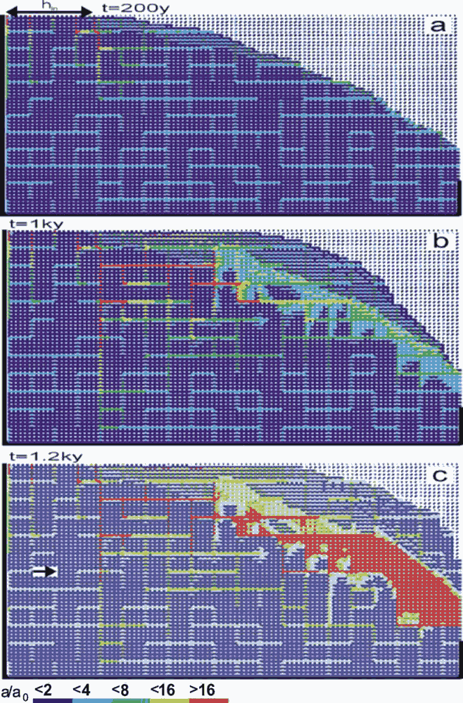
Fig. 32. Evolution of an aquifer with combined - constant recharge and constant head - boundary conditions and a percolation network of prominent fractures appended to the dense fracture network. The initial aperture width of prominent fractures is 0.02cm (light blue). Other parameters are the same as in Fig. 28. a) 0.2ky, b) 1ky, c) 1.2ky.
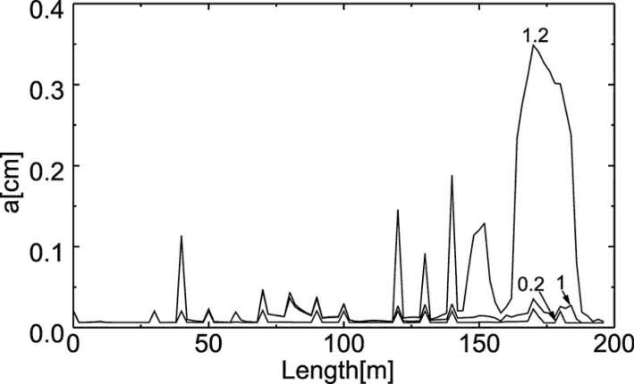
Fig. 33. Profiles of horizontal fractures along a cross-section as indicated by an arrow in Fig. 32c.
After 1.2ky breakthrough occurs (Fig. 32c), with prominent fracture aperture widths on the order of a few millimetres. To illustrate the distribution of fracture widths as they evolve in time, Fig. 33 depicts these along a horizontal cross-section as indicated by an arrow in Fig. 32c. The widening of the fracture accelerates by feedback and consequently the discharge through the aquifer shows the characteristic breakthrough behaviour. This event terminates the early evolution of the aquifer. The constant head condition breaks down and must be replaced by constant recharge. Flow becomes turbulent. Nevertheless, the complicated pattern of vertical and horizontal conduits and a high permeability region close to the spring will design the future structure of the mature karst aquifer. It should be stressed at that point, that constant head conditions are crucial for the evolution of such complicated structures as shown in Fig.32.
Another point of interest is that two processes proceed simultaneously: The evolution of conduits along the prominent fractures and creation of increasing permeability in the continuum, as shown by the red region in Fig 32c. Such behaviour cannot be obtained if dissolutional widening is restricted to the prominent fractures.
4.3 Time dependent boundary conditions: down cutting of the cliff
In nature the boundary conditions are changing during the evolution of a karst aquifer. The precipitation rate Q, the chemical parameters of the inflowing solution and also the hydrological boundary conditions may alter. All these variations can be applied to the model presented. We present a case where the base level of an aquifer is down cut during the evolution.
In a first scenario we assume that a ”sudden” incision of a valley lowers the base level. This is presented in Figs.34 a and b. The model is the same as used in Fig.31 but the position of base level is kept at 15m during the first 10ky and than it is down cut to 25m immediately. In Fig. 34a, which shows the situation at 9.8ky, a water table cave has developed and as in Fig.31 the system of conduits evolves below the base level.
After the down cutting the WT adopts to the new base level in a short time. This is presented in Fig.34b. After 11ky a new water table cave is already evolving. Between both base levels the hydraulic conductivity is relatively small since the WT has dropped fast due to the phreatic loops which have evolved prior to down cutting.
Probably more realistic than the step down cutting is a gradual down cutting. Such a scenario is shown on Fig.35. The initial base level is almost at the top of aquifer and is being lowered in steps of two nodes (1m) every 5ky. The mechanisms are similar to those for the step down cutting. The formation of phreatic conduits below base level forces the WT to adapt promptly to the temporary base level. Fig.35a and b show the aquifer at 6ky and 12ky, respectively. The vadose zone exhibits a relatively high permeability since the region of fast widening at the WT was gradually lowered together with the slow down cutting. A slower down cutting produces higher permeability in the vadose zone.
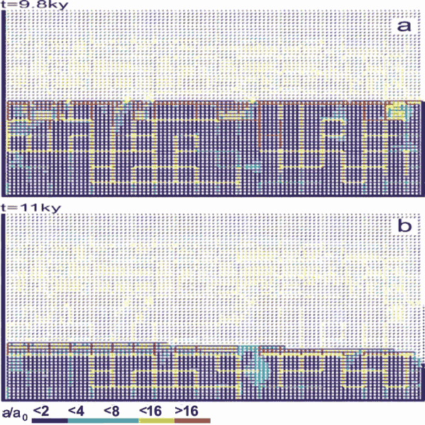
Fig. 34. Evolution of an aquifer with a net of prominent fracture under constant recharge condition with step down cutting of the base level.

Fig. 35. Evolution of an aquifer with a net of prominent fracture under constant recharge condition with gradual down cutting.
5. Conclusion
The basic element in modelling the early evolution of karst is a single 1-dimensional fracture which is widened by dissolutional attack of calcite-aggressive water. Under constant head conditions flow increases slowly at the beginning but then is enhanced dramatically and breakthrough occurs. The breakthrough times depend on the initial aperture width, the length and the hydraulic head acting on the entrance of the fracture. But they also depend on chemical parameters ceq, kn, n, which determine the dissolution kinetics. When these chemical parameters vary within a single fracture, f.i. ceq by injection of subterranean carbon dioxide or kn and n by varying lithology of the rock comprising the fracture, breakthrough times are changed significantly. Thus even for one-dimensional systems a great variety of boundary conditions determines the time scale of karst evolution.
A further step to model karst is the combination of one-dimensional fractures into a two-dimensional net either on length and breadth or on length and depth. By this way two-dimensional projections of karst aquifers can be modelled. In such nets due to the interaction of flow one-dimensional fractures can inject flow into this net and therefore enhance dissolutional widening by increased input flow of calcite aggressive solution. Consequently a prominent fracture embedded into a net of narrow fractures can exhibit breakthrough much earlier than if it were isolated. Furthermore boundary conditions in networks become more complex. Differing chemical compositions of input waters at various input regions cause mixing corrosion, where those waters mix, deep in the aquifer. This creates increased permeability which attracts further flow and directs conduits towards such regions. Therefore solely by chemical boundary conditions of the input waters karst aquifers with or without mixing corrosion (i.e. with or without differing chemical composition of the inflowing water) will develop entirely different. A large impact to the evolution of cave systems is caused also by different rock lithologies within the aquifer. Finally the hydrological boundary conditions, i.e. constant head inputs and their location and/or constant recharge to the surface of the aquifer exert significant influence.
Due to our lack of knowledge on all these various boundary conditions and their change in time it is not possible to explain a specific cave system by modelling. The aim of karst modelling is to understand the processes operating in the evolution of karst aquifers.
References
Beek, W.J. and Mutzall, K.M.K. 1975. Transport Phenomena. New York, Wiley.
Breznik, M. 1998. Storage reservoirs and deep wells in karst regions. Rotterdam ,A.A. Balkema, 251.
Buhmann, D. and Dreybrodt, W. 1985. The kinetics of calcite dissolution and precipitation in geologically relevant situations of karst areas: 2. Closed system. Chem. Geol. 53, 109-124.
Clemens, T., Huckinghaus, D., Sauter, M., Liedl, R. and Teutsch, G. 1997. Modelling the genesis of karst aquifer systems using a coupled reactive network model. In: Hard Rock Geosciences. Colorado, IAHS Publ. 241, 3-10,
Clemens, T., Huckinghaus, D., Sauter, M., Liedl, R. and Teutsch, G. 1996. A combined continuum and discrete networkreactive transport model for the simulation of karst development. In: Calibration and Reliability in Groundwater Modelling. Colorado, IAHS Publ 237, 309-318.
Clemens, T., Huckinghaus, D., Liedl , R. and Sauter, M. 1999. Simulation of the development of larst aquifers. The role of epikarst. Int. Journal of Earth Sciences, 88, 157-162.
Dreybrodt W. 1988. Processes in karst systems - Physics, Chemistry and Geology. Springer Series in Physical Environments 4, Berlin - New York, Springer, 288 p.,
Dreybrodt, W. 1990. The role of dissolution kinetics in the development of karstification in limestone: A model simulation of karst evolution. Journal of Geology 98, 639-655
Dreybrodt, W. 1996. Principles of early development of karst conduits under natural and man-made conditions revealed by mathematical analysis of numerical models. Water Resources Research 32, 2923-2935.
Dreybrodt, W., and Gabrovsek, F. 2000. Dynamics of the evolution of a single karst conduit. In: Klimchouk, A., Ford, D.C., Palmer, A.N. and Dreybrodt, W., (Eds.), Speleogenesis: Evolution of karst aquifers. Huntsville, Nat. Speleol. Soc., 184-193.
Dreybrodt, W. and Siemers, J. 2000. Cave evolution on two-dimensional networks of primary fractures in limestone. In: Klimchouk, A., Ford, D.C., Palmer, A.N. and Dreybrodt, W., (Eds.), Speleogenesis: Evolution of karst aquifers. Huntsville, Nat. Speleol. Soc., 201-211.
Eisenlohr, L., Madry, B. and Dreybrodt, W. 1997. Changes in the dissolution kinetics of limestone by intrinsic inhibitors adsorbing to the surface. In: Proceedings of the 12th Int. Cong. of Speleology , La Chaux de Fonds, Switzerland, Vol II, La Chaux de Fonds, Switzerland, 81-84,
Eisenlohr L., Meteva, K., Gabrovsek, F. and Dreybrodt, W. 1999. The inhibiting action of intrinsic impurities in natural calcium carbonate minerals to their dissolution kinetics in aqueous H2O-CO2 solutions. Geochimica et Cosmochimica Acta 63, 989-1002.
Ford, D.C. and Williams, P.W. 1989. Karst geomorphology and hydrology. London, Unwin Hyman, 601 p.
Gabrovsek, F. 2000. Evolution of early karst aquifers: From simple principles to complex models. Ljubljana, Zalozba ZRC, 150 p.
Gabrovsek, F., Menne, B. and Dreybrodt, W. 2000. A model of early evolution of karst conduits affected by subterranean CO2 sources. Environmental Geology 39, 531-543.
Gabrovsek, F. and Dreybrodt, W. 2000. The role of mixing corrosion in calcite aggressive H2O-CO2-CaCO3 solutions in the early evolution of karst aquifers. Water resources research 36, 1179-1188.
Gabrovsek,F., and Dreybrodt, W. 2001. A model of the early evolution of karst aquifers in limestone in the dimensions of length and depth. J. Hydrol 240, 27-34.
Incropera, F. and DeWitt, D. 1996. Fundamentals of Heat and Mass Transfer. 4rd edition, New York, John Wiley & Sons, 912 p.
Kaufmann, G. and Braun, J. 1999. Karst aquifer evolution in fractured rocks. Water Resources Research 35, 3223-3238.
Kaufmann, G. and Braun, J. 2000. Karst aquifer evolution in fractured, porous rocks. Water Resources Research 36, 1381-1391.
Liu Z. and Dreybrodt W. 1997. Dissolution kinetics of calcium carbonate minerals in H2O-CO2 solutions in turbulent flow: The role of the diffusion boundary layer and the slow reaction . Geochimica et cosmochimica acta 61, 2879-2889.
Lowe, D.J., and Gunn, J. 1997. Carbonate speleogenesis: An inception horizon hypothesis. Acta Carsologica 26 (2), 457-491.
Plummer, L.N., Parkhurst, D.L., and Wigley, T.M.L. 1978. The kinetics of calcite dissolution in CO2 systems at 25oC to 60oC and 0.0 to 1.0 atm CO2. American Journal of Science 278, 179-216.
Rhoades, R. and Sinacori, M.N. 1941. The pattern of ground-water flow and solution. Journal of Geology 49, 785-794.
Romanov, D., Dreybrodt, W. and Gabrovsek, F. 2002a. Interaction of fracture and conduit flow in the evolution of karst aquifers. In: Martin, J.B., Wicks, and Sasowsky I.D. (Eds.), Proceedings of the Symposium on Karst Frontiers: Florida and Related Environments. KWI Special Publication No. 7.
Romanov, D., Gabrovsek, F. and Dreybrodt, W. 2002b. The impact of hydrochemical boundary conditions on the evolution of karst aquifers in limestone terrains. Submitted to Journal of Hydrology.
Sauter, M. 1993. Double porosity models in karstified limestone aquifers: field validation and data provision. In: Gultekin, G., Johnson, I.A., (Eds.), Hydrogeological Processes in Karst terraines. IAHS Publication 207, 261-279.
Siemers, J. and Dreybrodt, W. 1998. Early development of karst aquifers on percolation networks of fractures in limestone. Water resources research 34, 409-419.
Swinnerton, A.C. 1932. Origin of limestone caverns. Geological Society of America Bulletin 34, 662-693.
Svensson, U. and Dreybrodt, W. 1992. Dissolution kinetics of natural calcite minerals in CO2 -water systems approaching calcite equilibrium. Chem. Geol. 100, 129-145.